PongBot

A room inside any building in the real world would have obstacles, such as walls and furniture, which the robot would need to navigate around. A straight shot from start to finish isn’t possible. So, the robot runs through a path planning algorithm before it starts to move, and only then drives on that path from start to finish, sticking as close to the path as possible.

A Star Path Planning

A variant of the A Star shortest paths algorithm is used to get the shortest path from the robot’s current location to the predicted sound source location given by the acoustics system. They're represented here by a green dot and an X respectively.

PID Actuation and Path Tracking

A PID controller, parameterized by the translation and rotation errors between the robot's current state and goal state, is used to move the robot from its current location to the sound source.

The final path given by the A Star algorithm shown above is essentially a list of straight paths connected together by corner points. This list of corner points is what gets sent between the path finding and PID controller ROS nodes. For each corner point, the robot will use the PID controller to drive to it, and make a smooth transition between the previous straight shot and the next one. This is what gives the stop/start behavior seen in the video on the right. This sequential completion was made to be modular with the FSM; for example, splitting up the path into many smaller paths lessens the difficulty of implementing a basic obstacle detection.

Preloading the Map

An assumption we had was that the base map (without extra obstacles) would be preloaded onto the robot before it begins its collection tasks. Under a lot of circumstances, however, this might not be the case, so dynamic path planning would be an ideal feature to add.

Corner to Corner

With our FSM, we had to trade smooth driving with modularity, however, this is something that could be easily fixed with a better driving control such as this one. Both the above and left gif can be found on this PythonRobotics repo.

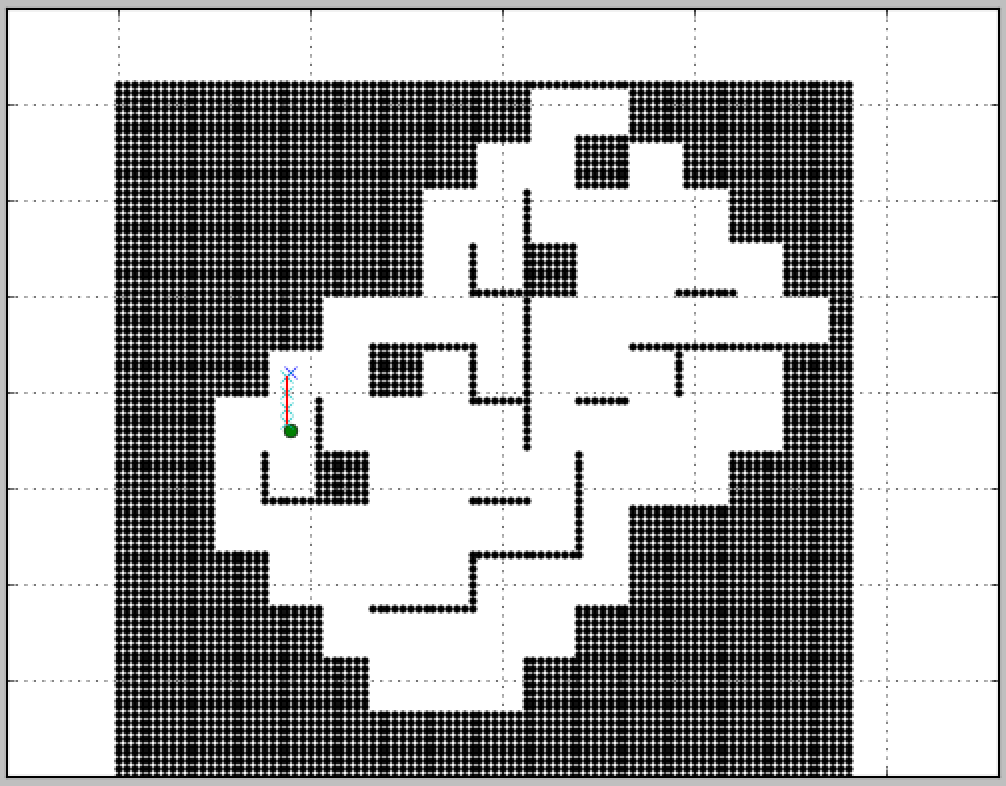
A Star Tradeoffs

Many optimizations were made for the A Star algorithm to work as quickly as it does, such as decreasing the resolution of the obstacle array (points which define the walls of the map). Above is the result of too much image resolution reduction. We had to find a nice balance between reducing the number of points A Star had to traverse over, and keeping the obstacles well defined.