PongBot

Assumptions

In order to get a basic application working, we needed to make several assumptions on the audio side of things. In particular, we assumed:

• A low reverb environment (controlled recording room type settings)
• Minimal physical interference of our audio source by objects in the room
• Minimal noise produced by objects in the room
• Stationary audio source

These assumptions are invalid in many environments, however it is necessary to first track locations using the above assumptions. Without the above conditions, we are prone to many sources of interference in our signal, but there are many methods we can use to eventually eliminate these assumptions, which can be found below in the future considerations section.

Audio Simulation

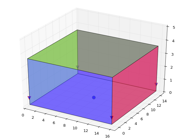
We decided to get our data for our PongFinder in a simulated environment. For this we used pyroomacoustics, an 3D acoustic simulation package based in python. This allows us to create a simple shoebox type room given certain parameters (dimensions, wall materials, etc.). We can then place sources (through audio files) and sinks (microphones) throughout our room. Although the simulation occurs in 3D, we can place our sources and sinks all close to the floor, in order to reduce our future approach for mathematical sourcing to a 2D problem. Our room can be seen in the above figure, with our audio source playing on the floor in the middle of the room, with 4 microphones, one at each corner of the room.

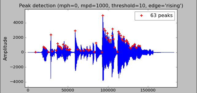
Once we're finished setting up our room, we can run our simulation. This represents the given audio file playing at it's location within the room and the recording of that audio by each microphone. This recording can be represented by an array of intensities over a period of time and it is visualized below. The detection of important peaks can be seen as the red crosses.

Source Localization

Essentially what we are doing is the same process as cellphone triangulation by cell towers, but here we are using the propagation of sound instead of EM waves. We know the speed of sound, but we do not know each absolute time it took for the wave to get to each individual microphone. However, since we have a signal array from each microphone, we can calculate the relative time the sound took to travel to each microphone compared to the others. This gives us a system of equations which gives us the distance of the source to each microphone compared to the others. We can then iterate over these equations, starting from a very small distance, slowly increasing until we can converge onto a small enough area. For an enclosed space, we need a minimum of 3 microphones for this to work, however we chose 4 both to minimize error and to have a backup in case one of the signals is becomes unusable for any reason (noisy data, faulty mics). Below is a visualization of the base case of our iterative process, a square room with our signals converging on the point source located at the center of the room.

Using this iterative process does come with it's challenges. For each iteration, our goal is to find the intersections of each function if there are any. These intersections represent possible point sources, but since our signal data is never 100% perfect or continuous, we generally can't get one intersection for all functions. So our solution is to use a custom gradient function to minimize the area covered by the polygon created by connecting the intersections. The reason we need to create a customized function is that each case varies in how the intersections approach the point. The case below shows a point source slightly away from the center. We can see that the distance visualised from the left microphones are smaller than the right microphones, since each circle's size is proportional to the time taken for the sound to travel. This results in the intersections between the top-left and bottom-left microphones to take longer to appear in the room compare to the other intersections. This effect is exagerrated more when the sources are closer to the walls and it required more careful iteration to get to our source. Overiteration was also a problem, if we accidently iterated over our source location, we would get extra intersections that aren't physically possible. The customisability of our own naive gradient function gave us the ability to work around these problems while also giving us the option to account for errors by a microphone or even accounting for additional microphones. We were able to localize all sources within approximately a 0.1 x 0.1 m^2 area.

Simulation Tradeoffs

Arguably the biggest decision we made for developing audio source triangulation was using audio simulation software instead of actual hardware. By choosing a simulated environment, we are deciding not to take into account possible issues we would face when transitioning to hardware. However for the scope of this project, using simulations was definitely worth it, because it allowed for repeated testing and the development of a functional triangulation method without having to worry about the physical elements. Nevertheless, when considering next steps in our work, it is important to at least perform occasional tests with hardware as our backend functionality progresses, so that we can address critical issues as they come. We can perform these tests as we progress with topics that are listed below.

Future Considerations

Losing Our Assumptions -

A large portion of future work will involve addressing issues regarding our assumptions, so that we can expand into working in more realistic environments.

• Reverb is additional noise that comes from echoes in our environment and it is the most important real world effect we need to take into account.
• There are many music production packages we can work with to digitally remove reverb, such as Zynaptiq Unveil and iZotope RX 6 De-Reverb.
• Physical interference is our next problem, this involves the blocking of sound waves by large objects that are close to the floor, like furniture.
• An easy fix to this is simply adding microphones to cover the entire room without interference and accounting for this in our software.
• Noise produced by either people or electronics like speakers or TV's are another important consideration.
• We can place microphones closer to the sources we want to disregard, then we can remove this from the signal that our floor mics are tracking.
• Tracking moving sources is another useful functionality we can implement.
• For sources with predictable movement (bouncing balls), we can anticpate locations using a physics simulation, for less predictable objects, ML.
• Physical Environment
• As previously mentioned, transitioning to testing with hardware in real environments as we add functionality is critical.

Expanding our Analysis -

While dealing with the issues with constrained environments, we can also expand on the algorithms and tools we use after we have obtained our signals. This involves creating custom algorithms to more appropriately track our errors, using Fourier Analysis to isolate our desired audio sources, and even incorporating Machine Learning in our triangulation methods. Our ultimate goals are to localize an audio source in any situation without any constraints on conditions and without having to customize our algoritms for each individual environment, and as you can see, there are many directions we can take this in!